The Probability That X Is Between 0.5 and 1.5 Is

If we assume the probabilities of each of the values is equal then the probability would be PX2frac15. What is the probability that the series lasts only 4 games.

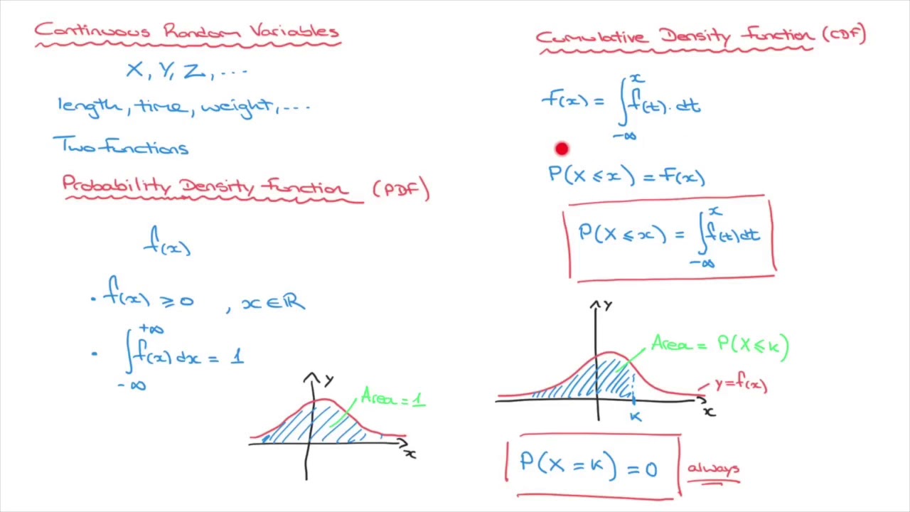
Continuous Probability Distributions Random Variables

80 90 100 110 120 130 140 150 160 0 5 10 15 20.

. Thus in problems where OLS breaks down due to correlation of right-hand-side variables and the disturbances you can use IV to get consistent estimates provided you can find proper instruments. Return probability estimates for the test data X. The measure computes the cosine of the angle between vectors x and y.

The survival probability is 08095038 if Pclass were zero intercept. If we assume the probabilities of all the outcomes were the same the PMF could be displayed in function form or a table. N t number of participants who are event free and considered at risk during interval t eg in this example the number alive as our outcome of interest is death D t number of participants.

Ü Ü Ü. We can define the probabilities of each of the outcomes using the probability mass function PMF described in the last section. How to convert logits to probability.

This constitutes a Nash equilibrium in mixed strategies. For instance as defined by Koza non- terminal primitives are selected for 90 of the crossover points and terminals for 10 so termpb should be set to 01. The probability of the National League team winning 4.

Between H and T with probability ½. The profile is a mixedstrategy Nash equilibriumif and only if playing is a best response to. Consider a mixed strategy profile 5 6 á where Üis a mixed strategy for player.

Lets look first at the simplest case. Note that because the cosine similarity measure does not obey all of the properties of Section. Nola fouled out to right Kim to third.

If we assume the probabilities of each of the values is equal then the probability would be PX2frac15. 80 90 100 110 120 130 140 150 160 0 5 10 15 20 25 P e r c e n t POUNDS 968 1278 95 of 120 95 x 120 114 runners In fact 115 runners fall within 2-SDs of the mean. The idea behind 5 is that W and are orthogonal in the popul ation a generalized.

The estimate is based on a normal kernel function and is evaluated at equally-spaced points xi that cover the range of the data in xksdensity estimates the density at 100 points for univariate data or 900 points for bivariate data. The closer the cosine value to 1 the smaller the angle and the greater the match between vectors. Parameters X array-like sparse matrix of shape n_samples n_features or n_samples.

The parameter termpb sets the probability to choose between a terminal or non-terminal crossover point. This can occur if one team wins the first 4 games. Grahams number is a tremendously large finite number that is a proven upper bound to the solution of a certain problem in Ramsey theory.

A cosine value of 0 means that the two vectors are at 90 degrees to each other orthogonal and have no match. Therefore the probability that a particular team wins a particular game is 05. In basic probability we usually encounter problems that are discrete eg.

See probability by outcomes for more. We can define the probabilities of each of the outcomes using the probability mass function PMF described in the last section. If R W Xn converges in probability to a nonsingular matrix and R W n p 0 then b IV p β.

Fit X y source Fit the k-nearest neighbors classifier from the training dataset. 0 5 10 15 20 25 P e r c e n t POUNDS 1123 1278 1433 68 of 120 68x120 82 runners In fact 79 runners fall within 1-SD 155 lbs of the mean. Score X y sample_weight Return the mean accuracy on the given test data and labels.

We use the following notation in our life table analysis. If the matrix is regular then the unique limiting distribution is the uniform distribution π 1N 1NBecause there is only one solution to π j k π k P kj and σ k π k 1 when P is regular we need only to check that π 1N 1N is a solution where P is doubly stochastic. Geometric probability is a tool to deal with the problem of infinite outcomes by measuring the number of outcomes geometrically in terms of length area or volume.

Nola flied out to center. Nola homered to left 393 feet. Fxi ksdensityx returns a probability density estimate f for the sample data in the vector or two-column matrix x.

When the nodes are strongly typed the operator makes sure the second node type corresponds to the first node type. However you cannot just add the probability of say Pclass 1 to survival probability of PClass 0 to get the survival chance of 1st class passengers. Consider a doubly stochastic transition probability matrix on the N states 0 1 N 1.

We first define the notation and then use it to construct the life table. The outcome of a dice roll. Üfor each Ü Ü Fact 1 about mixedstrategy Nash EquilibriumA.

It is named after mathematician Ronald Graham who used the number as a simplified explanation of the upper bounds of the problem he was working on in conversations with popular science writer Martin Gardner. However some of the most interesting problems involve. After you insert your data set it calculates the mean and standard deviation of data automatically in the background and delivers the very precise value for the coefficient of variation.

Nola struck out looking. Nola struck out swinging. If we assume the probabilities of all the outcomes were the same the PMF could be displayed in function form or a table.

Coefficient of Variation calculator can be used to calculate the coefficient of variation in the given data set by evaluating the ratio between standard deviation and mean of that set. Set_params params Set the parameters of this estimator. Instead consider that the logistic regression can be interpreted as a normal.

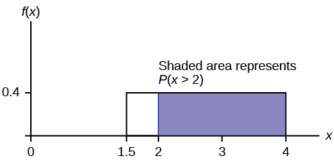
The Uniform Distribution Introductory Statistics

1

1

1